Better Living Through (Flavor) Chemistry Part 2 – Read Between (or Beneath) the Lines

What if I told you that the terpenes chromatogram I showed you last time isn’t what it appears to be? Sure, it looks like a regular old chromatogram on the surface, but lurking beneath that innocuous line is a plethora of vacuum ultraviolet absorbance spectral data, the beating heart of our technology and a power that would drive you into a Lovecraftian madness were you to glimpse it directly. But we’ve bent this Great Old One to our will, ignoring trifles like co-elutions and reshaping the chromatographic landscape at will. A power both beautiful and terrible! Muahahaha! Sorry, sometimes the power still gets the best of us.

In Part 1 we deliberately compressed the chromatography for our terpenes standard and forced some co-elutions. We were able to do this because we can visually distinguish the absorbance spectra of structural isomers. In Part 2 of Better Living Through (Flavor) Chemistry, we’ll utilize these unique absorbance spectra and dive into the chromatographic data to spectrally deconvolve some of these co-eluting isomers.

Figure 1 shows five monoterpenes eluting in a 0.2-minute time window, four of which are isomers. However, remember that our chromatographic data is just a visual representation of the absorbance data. Let’s take a closer look at the absorbance data in four regions along this cluster of peaks and see what the spectra show us.

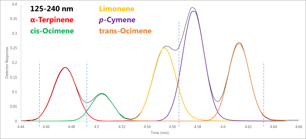
Figure 1. Using the raw spectral data that are visually represented by this chromatogram, we can de-convolve these co-eluting peaks, four of which are structural isomers.

In Region 1, where we expect to only see the single analyte α-terpinene, that’s exactly what we find, and a 0.999 spectral fit definitively supports this claim (Figure 2).

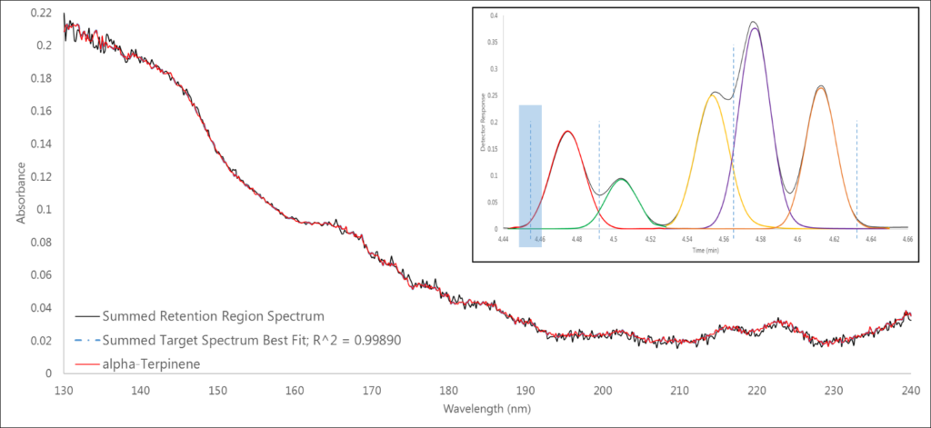
Figure 2. Region 1 (highlighted in blue) shows a single analyte spectrum match of α-terpinene.

The second region is our first co-elution – α-terpinene and cis-ocimene, which are monoterpene isomers (Figure 3). Again, we have a 0.999+ spectral fit, which gives us confidence in our data. But how can we be so confident? Remembering Beer’s Law, the measured absorbance is linearly proportional to the amount of analyte going through the flow cell. Thus, the individual analyte library spectra can be summed to fit the area of the captured absorbance spectrum.

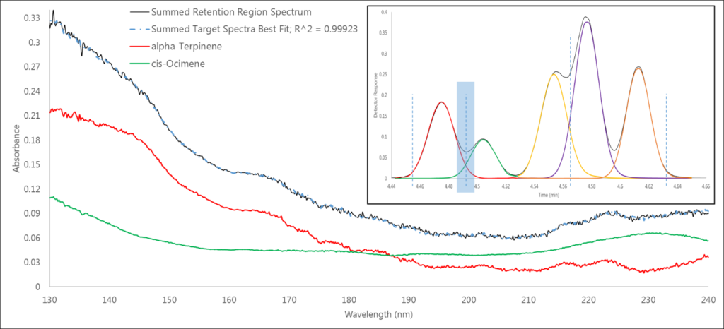
Figure 3. In this co-elution of α-terpinene and cis-ocimene in region 2, we can see that the measured spectrum is simply the sum of the absorbances of the individual spectra of these isomers.

The third region is another co-elution (Figure 4), this time between limonene and p-cymene (and another 0.999+ fit). While these aren’t isomers, this deconvolution does highlight how we can visually see that spectrum A plus spectrum B equals our best fit spectrum.

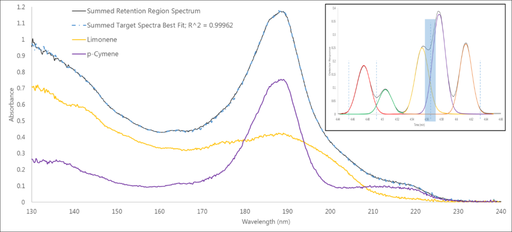
Figure 4. Region 3 has another co-elution, between limonene and p-cymene, in which we can more clearly see that the component spectra can be summed to match the measured absorbance spectrum.

Finally, we’re back to a single analyte spectrum match in the fourth region, which in this case is a 0.998 fit to trans-ocimene (Figure 5). OK, so maybe I embellished the power of the spectral data just a bit; I hope you haven’t been driven mad quite yet. But I also hope you see that the absorbance data is powerful enough to overcome co-eluting isomers, which is no small feat!

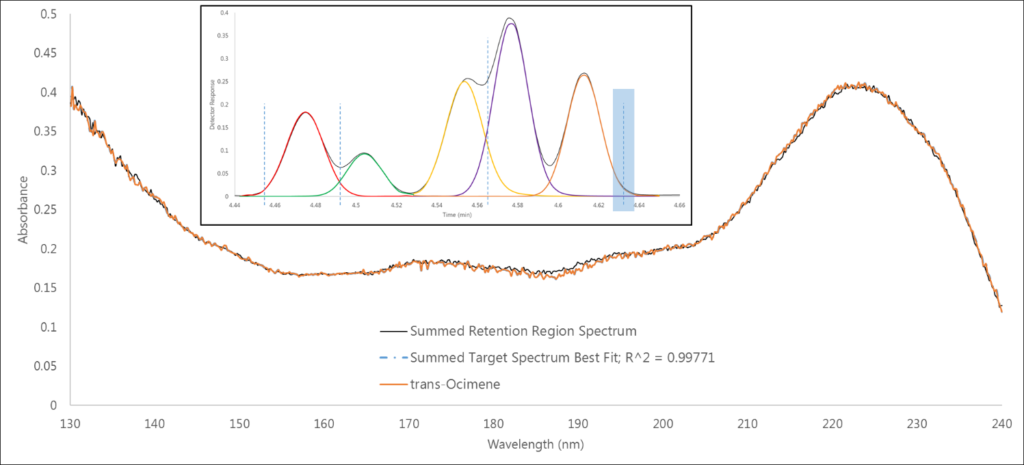
Figure 5. In region 4 we’re back to a single analyte spectrum match, this time of trans-ocimene.

Next time we’ll get into some real samples with a look at terpenes in essential oils!