Response Factor Scalability & VUV Consistency

The last time I wrote, I gave the wackiest introduction from Plato’s Academy and then launched into vacuum ultraviolet (VUV) spectroscopy response factors (RFs), spectral filters (SFs) and deconvolution. This month, I would like to start off by singing a song. Thank you. I hope you enjoyed it too. It was, quite possibly, the finest rendition of The Sounds of Silence I’ve ever had the pleasure of giving.

Moving on then. I’ll spend the rest of this blog tickling the keyboard of this sluggish laptop rather than your ears (please make him stop!). I want to spend more time on:

• 1. SFs and RFs and show that from one set of RFs at a given SF
• 2. one can calculate relative RFs (RRFs) and then
• 3. theoretically determine the RRF at any other SF you wish purely from the spectra of the analytes of interest.

First things first; who the heck cares? Well, it is widespread practice in chromatography to monitor multiple signals from your detector assuming it has the capacity to do so. Examples include GC-MS SIM, GC-MS/MS, GC-VUV and the HPLC equivalents (ESI-MS, etc., and DAD). The ability to relate these signals to one another by a simple proportionality constant would be great. While I do not have enough experience to know whether this is possible with all techniques, I know it is very reliable in GC-VUV.

1. SFs and RFs

Recall that a spectral filter is simply a software feature that extracts a wavelength region from the default full wavelength spectra (125 – 240 nm) collected using our VUV detector. It can be plotted real-time during data acquisition, or it may be introduced post-run. Figure 1 shows a snapshot of the post-run SF development tool called Filter Integrator.

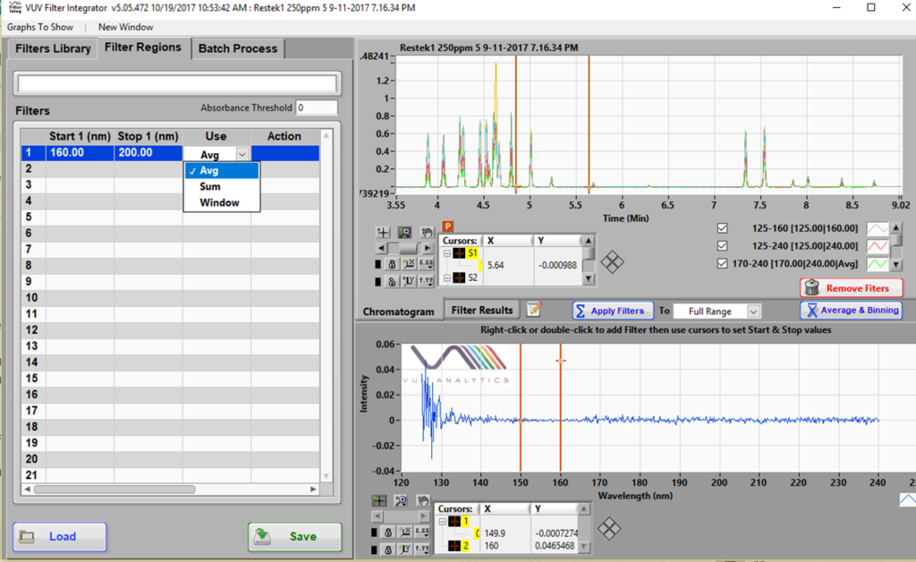
Figure 1.  Spectral Filters can be prepared using the Filter Integrator part of the VUV software.  An example where a 160 – 200 nm SF is being made is shown here.

SFs can be calculated either as the average (Avg) or sum of the absorption values in the given range. There is very little difference between the two. While the latter will give a higher signal, the noise will scale proportionately as well and will result in much the same S/N as the Avg would. I will not get into the Window function here, even though it is the OS on my laptop… High yo (drum beat)! The Avg vs. Sum calculation is important for the theoretically determined RRFs I alluded to above. More about this later. All the data used here has the Avg calculation for SFs.

Overlaid chromatograms using several SFs are shown in Figure 2 (kudos to my colleague Alex who generated this fine data).  See his blogs at Better Living Through (Flavor) Chemistry Part 1 – We Don’t Need No Separation, We Don’t Need No Flow Control and Better Living Through (Flavor) Chemistry Part 2 – Read Between (or Beneath) the Lines.  Here you can see that the 170 – 240 nm SF has a lower response than the 135 – 160 nm. In other words, each SF has its own RF for a given concentration.

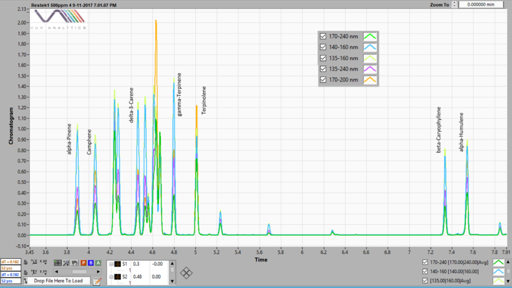
Figure 2.  A chromatogram of a 500 ppm terpene standard mix run by static headspace – GC-VUV. Five different spectral filters are shown, 170 – 240, 140 – 160, 135 – 160, 135-240 and 170 – 200 nm, each indicating different response factors.

2. Calculation of RRFs

This is practically the shortest part of this blog as it’s a universal practice across many analytical disciplines. Before I embark on this, I need to have a reference analyte (unfortunately I did not have an internal standard here, but that would’ve been the logical choice) and SF. I am going to the invoke the power of the chromatographer and designate alpha-humulene as my reference analyte and use the 140 – 160 nm SF as my reference. Done. Next, I will show the experimentally determined RRFs for each of the SFs relative to the reference analyte for a range of standards from 1 – 250 ppm (here the RF is the slope of the calibration curve). The results of this are shown in Table 1.

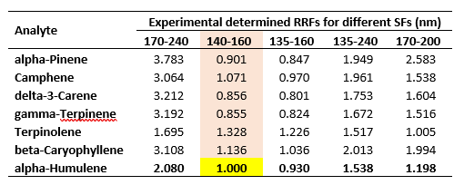
Table 1.  Results of the experimentally determined RRFs for a range of terpene standards from 1 – 250 ppm.

3. Theoretical determination of RRFs from VUV absorbance spectra.

In the beginning, I referred to the widespread practice of monitoring multiple signals from an appropriate detector where each signal would have its own characteristic RF.  The question is whether these RFs can be related to each other or do they vary from day to day, sample to sample, instrument to instrument? In VUV I am confident the RRFs are the same (within narrow limits). The reason is because the spectra are constant for a given set of flow cell conditions. The spectra rise and fall evenly across a chromatographic peak. The spectra for the seven terpenes above are shown in Figure 3. Incidentally, I would be remiss not to point out the spectral differences in the structural isomers alpha-pinene, delta-3-carene, gamma-terpinene and terpinolene, while their mass spectra are very similar (see also Alex’s work referenced above).

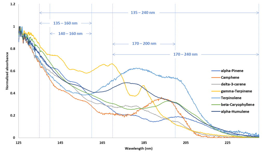
Figure 3. VUV spectra for seven terpenes with five, relevant SF regions demarcated.

Because these spectra behave in a consistent manner, we can use the 140 – 160 nm RRF data to calculate RRFs for all the other SFs. To put it in other words, if the RRF for a given compound is known for a SF, it is known for every other SF provided its spectrum is well defined in that region (or to spoof Tolkien’s refrain, “One RF to rule them all…”). My colleague James has a blog on adding spectra to the library and stresses the importance of making sure that the spectrum is pure and well defined, Let’s Chat About YOUR Absorbance Spectra Library.  Jimmy, are you listening?

Regardless of whether Jimmy is listening, I know you are, my avid reader. The theoretical determination of the RRFs uses scaling factors derived from the above spectra. Perhaps an example will do. Suppose I want to express my seven terpene RRFs determined for the 140 – 160 nm SF in 170 – 200 nm. This is easily done by multiplying the RRFs at 140-160nm by the scaling factor for 140 – 160 nm (i.e. the average (see section 1 on SFs and RFs above) absorption values for the above spectra, as shown, in the 140 – 160 nm wavelength range) followed by dividing by the scaling factor for 170 – 200 nm. Table 2 shows the scaling factors derived from the spectra in Figure 3.

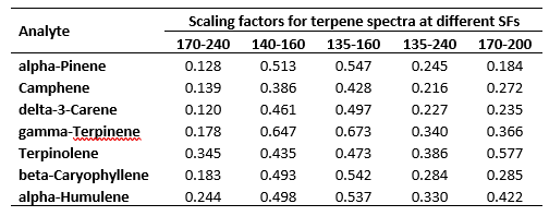
Table 2.  Scaling factors derived from the seven terpene spectra shown in Figure 3.

The results of applying these scaling factors as described are presented in Table 3 in the form of percent recoveries of the experimentally determined RRFs (Table 1).

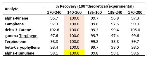
Table 3.  Percent recoveries of experimentally determined RRFs in Table 1 using spectral scaling factors.

The recoveries are excellent, ranging from 95 – 105 %. Most of the recoveries fall within 97 – 100 %.